Introduction
The ancient olympic game was help at Olympia, Greece, from 776 BC through 393 AD. It returned after 1503 years. THe first modern olympic was held in Athenes, Greece in 1896. The ‘modern Olympics’ comprises all the Games from Athens 1896 to Rio 2016. Baron Pierre de Coubertin presented the idea in 1894.
There are two long periods without any Games between 1912-1920 and 1936-1948, corresponding to WWI and WWII.
Perhaps, the most significant benefit of visual analytics is to ease the understanding of complex data, while representing it in correct, concise, and appropriate way. This manuscript proposes a handy visualization analysis of Olympic games between 1896 to 2016, which comprises in four levels of design system. These four levels are;
- Characterization of the tasks and data in the vocabulary of the problem domain,
- Abstract into operations and data types,
- Design visual encoding and interaction techniques,
- Create algorithms to execute these techniques, efficiently.
This application utilizes concrete analysis examples and claim to provide efficient, effective, functional, and convenient model for users. Discussion, conclusion, future work are summarized along with requesting recommendation for improvement of the limitations, where it was surveyed in evaluation as another section.
Goal
- How participation changed over time?
- What nations own most medels in various discipline?
- female in Olympics
Data Characteristics
- events (summer and winter)
- sports level data
- atheletes level data
- excluded art competition (focused on atheletics)
Domain Problem Charactarization
Choosing an empiric dataset has a great impact on the quality of the project. After researching myriad types of dataset, 120 Years of Olympic game is considered for representation. Advantages of its dataset is not limited of being a large scale that spans between 1896 to 2016. Over the years of course to be able to show the medal counts in popular sports (basketball) and orphan sports (lacrosse) is some of the useful feature of the application. Last but not least, considering visual representation perspective and providing the best user experience, Olympic game dataset is found worth to study.
The application aims to attract users who have interest on Olympics and address their curiosity in a clear way. Although, detailed information is provided in the app, primary research question is dealt with the dominant countries in each sport type. Dataset is picked from Kaggle, which consists of two distinct tables, athlete_events and event_regions, to address the primary question.
App is consisted of five tabs, which are information about the Olympics, world and host city, top countries and athletes. One way to evaluate the shiny dashboard would be to set up an experiment where users asked which country got the most medals in different sports and examine if the answers are correct with the ground truth data.
Data/operation abstraction design
Two different data frames were used for creating dashboard. After exploring the dataset, it is decided not to remove any data, and instead data manipulation/transformation with the dplyr package was conducted to make it applicable and plausible.
Some variables, athlete’s age, weight, and height were not executed in shiny dashboard but are incorporated in the presentation for the overview.
Geospatial visual representation is reflected on world map.
Detailed observations such as name, sex, age, weight, team’s region, game type, location, season, medals and the year of the Olympics were also examined.
Both categorical (name, sex, team, region, year, city, and medal type), and numerical (athlete’s age, weight, and height) variables were utilized.
1. Athelete Events data
library("plotly")
library("tidyverse")
library("data.table")
library("gridExtra")
library("knitr")
library("gganimate")


# Load athletes_events data
data <- read_csv("Data/athlete_events.csv",
                 col_types = cols(
                   ID = col_character(),
                   Name = col_character(),
                   Sex = col_factor(levels = c("M","F")),
                   Age =  col_integer(),
                   Height = col_double(),
                   Weight = col_double(),
                   Team = col_character(),
                   NOC = col_character(),
                   Games = col_character(),
                   Year = col_integer(),
                   Season = col_factor(levels = c("Summer","Winter")),
                   City = col_character(),
                   Sport = col_character(),
                   Event = col_character(),
                   Medal = col_factor(levels = c("Gold","Silver","Bronze"))
                 )
)

glimpse(data)
## Observations: 271,116
## Variables: 15
## $ ID <chr> "1", "2", "3", "4", "5", "5", "5", "5", "5", "5", "6", "6…
## $ Name <chr> "A Dijiang", "A Lamusi", "Gunnar Nielsen Aaby", "Edgar Li…
## $ Sex <fct> M, M, M, M, F, F, F, F, F, F, M, M, M, M, M, M, M, M, M, …
## $ Age <int> 24, 23, 24, 34, 21, 21, 25, 25, 27, 27, 31, 31, 31, 31, 3…
## $ Height <dbl> 180, 170, NA, NA, 185, 185, 185, 185, 185, 185, 188, 188,…
## $ Weight <dbl> 80, 60, NA, NA, 82, 82, 82, 82, 82, 82, 75, 75, 75, 75, 7…
## $ Team <chr> "China", "China", "Denmark", "Denmark/Sweden", "Netherlan…
## $ NOC <chr> "CHN", "CHN", "DEN", "DEN", "NED", "NED", "NED", "NED", "…
## $ Games <chr> "1992 Summer", "2012 Summer", "1920 Summer", "1900 Summer…
## $ Year <int> 1992, 2012, 1920, 1900, 1988, 1988, 1992, 1992, 1994, 199…
## $ Season <fct> Summer, Summer, Summer, Summer, Winter, Winter, Winter, W…
## $ City <chr> "Barcelona", "London", "Antwerpen", "Paris", "Calgary", "…
## $ Sport <chr> "Basketball", "Judo", "Football", "Tug-Of-War", "Speed Sk…
## $ Event <chr> "Basketball Men's Basketball", "Judo Men's Extra-Lightwei…
## $ Medal <fct> NA, NA, NA, Gold, NA, NA, NA, NA, NA, NA, NA, NA, NA, NA,…head(data)## # A tibble: 6 x 15
## ID Name Sex Age Height Weight Team NOC Games Year Season
## <chr> <chr> <fct> <int> <dbl> <dbl> <chr> <chr> <chr> <int> <fct>
## 1 1 A Di… M 24 180 80 China CHN 1992… 1992 Summer
## 2 2 A La… M 23 170 60 China CHN 2012… 2012 Summer
## 3 3 Gunn… M 24 NA NA Denm… DEN 1920… 1920 Summer
## 4 4 Edga… M 34 NA NA Denm… DEN 1900… 1900 Summer
## 5 5 Chri… F 21 185 82 Neth… NED 1988… 1988 Winter
## 6 5 Chri… F 21 185 82 Neth… NED 1988… 1988 Winter
## # … with 4 more variables: City <chr>, Sport <chr>, Event <chr>,
## # Medal <fct>2. NOC Regions data
# Load data file matching NOCs with mao regions (countries)
noc <- read_csv("Data/noc_regions.csv",
                col_types = cols(
                  NOC = col_character(),
                  region = col_character()
                ))
glimpse(noc)
## Observations: 230
## Variables: 3
## $ NOC <chr> "AFG", "AHO", "ALB", "ALG", "AND", "ANG", "ANT", "ANZ", "…
## $ region <chr> "Afghanistan", "Curacao", "Albania", "Algeria", "Andorra"…
## $ notes <chr> NA, "Netherlands Antilles", NA, NA, NA, NA, "Antigua and …head(noc)## # A tibble: 6 x 3
## NOC region notes
## <chr> <chr> <chr>
## 1 AFG Afghanistan <NA>
## 2 AHO Curacao Netherlands Antilles
## 3 ALB Albania <NA>
## 4 ALG Algeria <NA>
## 5 AND Andorra <NA>
## 6 ANG Angola <NA>Encoding/Interaction design
Olympic games are globally played and thus the date revealed from it is interest of world map and the medal counts. Another interesting analysis is ranking of athletes and countries, which are represented with bar charts.
User friendly Shiny dashboard is very convenient to show visual representations interactively, and more specific questions make it reliable tool. Redundant visual representations may negatively affect its usefulness, where it is aimed to provide concise visualization with deep understanding.
1. Has the number of athletes, nations, and events changed over time?
# Load athletes_events data
data <- read_csv("Data/athlete_events.csv",
                 col_types = cols(
                   ID = col_character(),
                   Name = col_character(),
                   Sex = col_factor(levels = c("M","F")),
                   Age =  col_integer(),
                   Height = col_double(),
                   Weight = col_double(),
                   Team = col_character(),
                   NOC = col_character(),
                   Games = col_character(),
                   Year = col_integer(),
                   Season = col_factor(levels = c("Summer","Winter")),
                   City = col_character(),
                   Sport = col_character(),
                   Event = col_character(),
                   Medal = col_factor(levels = c("Gold","Silver","Bronze"))
                 )
)

# count number of athletes, nations, & events, excluding the Art Competitions
counts <- data %>%
  group_by(Year, Season) %>%
  summarize(
    Athletes = length(unique(ID)),
    Nations = length(unique(NOC)),
    Events = length(unique(Event))
  )
counts <- counts %>%
  mutate(gap= if(Year<1920) 1 else if(Year>=1920 & Year<=1936) 2 else 3)
p1 <- ggplot(counts, aes(x=Year, y=Athletes, group=interaction(Season,gap), color=Season)) +
  geom_point(size=2) +
  geom_line() +
  scale_color_manual(values=c("darkorange","darkblue")) +
  xlab("") +

  annotate("text",x=c(1916,1942),y=c(10000,10000),
           label=c("WWI","WWII"), size=4, color="red") +
  geom_segment(mapping=aes(x=1914,y=8000,xend=1918,yend=8000),color="red", size=2) +
  geom_segment(mapping=aes(x=1939,y=8000,xend=1945,yend=8000),color="red", size=2)
p2 <- ggplot(counts, aes(x=Year, y=Nations, group=interaction(Season,gap), color=Season)) +
  geom_point(size=2) +
  geom_line() +
  scale_color_manual(values=c("darkorange","darkblue")) +
  xlab("")
p3 <- ggplot(counts, aes(x=Year, y=Events, group=interaction(Season,gap), color=Season)) +
  geom_point(size=2) +
  geom_line() +
  scale_color_manual(values=c("darkorange","darkblue"))
grid.arrange(p1, p2, p3, ncol=1)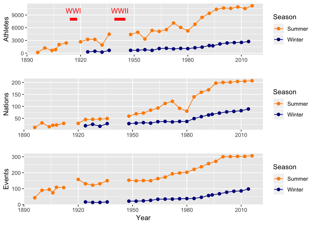
2. Which countries won the most medals (TOP 10)?
# count number of medals awarded to each Team
medal_counts <- data %>% filter(!is.na(Medal))%>%
  group_by(Team, Medal) %>%
  summarize(Count=length(Medal))

# order Team by total medal count
levs <- medal_counts %>%
  group_by(Team) %>%
  summarize(Total=sum(Count)) %>%
  arrange(desc(Total)) %>%
  select(Team) %>%
  slice(10:1)
medal_counts$Team <- factor(medal_counts$Team, levels=levs$Team)
medal_counts <- medal_counts %>% filter(Team != "NA")
# plot
ggplot(medal_counts, aes(x=Team, y=Count, fill=Medal)) +
  geom_col() +
  coord_flip() +
  scale_fill_manual(values=c("gold1","gray70","gold4")) +
  ggtitle("Historical medal counts from Competitions") +
  theme(plot.title = element_text(hjust = 0.5))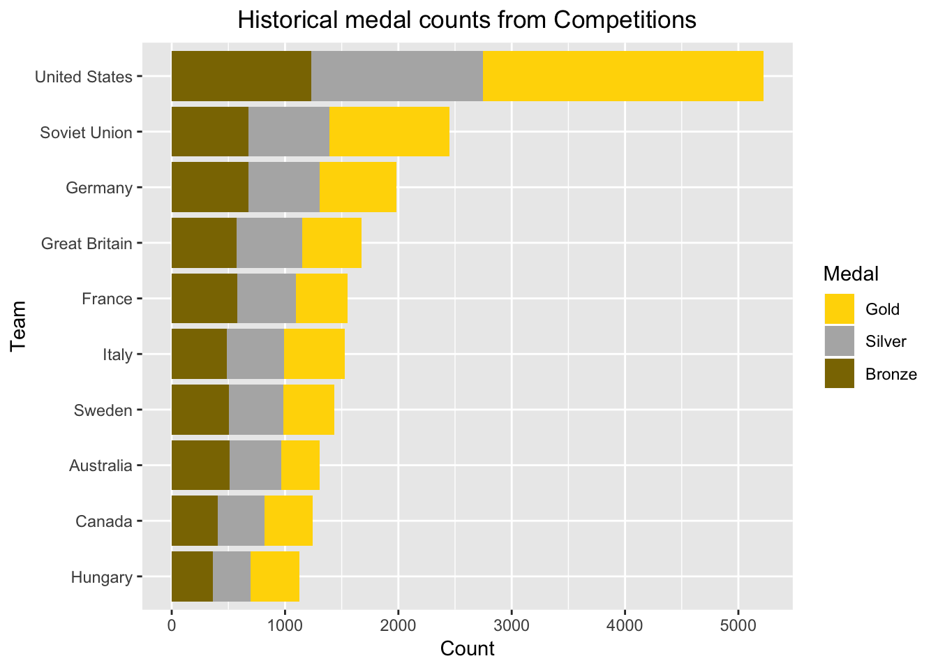
Top countries in Olympic games were found to be USA, Soviet Union, Germany, Great Britain, France, Italy, Sweden, Australia, Canada, Hungary. Another helpful information expresses that USA is dominant country in terms of gold, silver, bronze medals.
3.Which countries won the most medals- Map view
# Load data file matching NOCs with mao regions (countries)
noc <- read_csv("Data/noc_regions.csv",
                col_types = cols(
                  NOC = col_character(),
                  region = col_character()
                ))

medal_counts <- data %>% filter(!is.na(Medal))%>%
  group_by(NOC) %>%
  summarize(Count=length(Medal))

data_regions <- medal_counts %>%
  left_join(noc,by="NOC") %>%
  filter(!is.na(region))

world <- map_data("world")
world <- left_join(world, data_regions, by="region")
# Plot:
p <- ggplot(world, aes(x = long, y = lat, group = group)) +
  geom_polygon(aes(fill = Count, label= region)) +
  labs(title = "regions",
       x = NULL, y=NULL) +
  theme(axis.ticks = element_blank(),
        axis.text = element_blank(),
        panel.background = element_rect(fill = "navy"),
        plot.title = element_text(hjust = 0.5)) +
  guides(fill=guide_colourbar(title="medals")) +
  scale_fill_gradient(low="lightgreen",high="darkgreen")
4.Number of female and male over time
Despite the fact that male athletes were tremendously higher than the females, the latter one showed steep slope after 1980, where ultimately the difference was only around 2000 between them.
# Exclude art competitions from data (I won't use them again in the kernel)
data <- data %>% filter(Sport != "Art Competitions")

# Recode year of Winter Games after 1992 to match the next Summer Games
# Thus, "Year" now applies to the Olympiad in which each Olympics occurred
original <- c(1994,1998,2002,2006,2010,2014)
new <- c(1996,2000,2004,2008,2012,2016)
for (i in 1:length(original)) {
  data$Year <- gsub(original[i], new[i], data$Year)
}
data$Year <- as.integer(data$Year)

# Table counting number of athletes by Year and Sex
counts_sex <- data %>% group_by(Year, Sex) %>%
  summarize(Athletes = length(unique(ID)))
counts_sex$Year <- as.integer(counts_sex$Year)
Primary and secondry view findings
Please see the shiny dashboard. (https://anjali-bapat.shinyapps.io/Final_Project/)
Top countries in Olympic games were found to be USA, Soviet Union, Germany, Great Britain, France, Italy, Sweden, Australia, Canada, Hungary. Another helpful information expresses that USA is dominant country in terms of gold, silver, bronze medals.
Despite the fact that male athletes were tremendously higher than the females, the latter one showed steep slope after 1980, where ultimately the difference was only around 2000 between them.
USA athletes, Matt Biondi and Natalie Anne Coughlin win the most gold and bronze medals, respectively.
Only few countries (Canada, France, Norway, USA, Austria, Australia) showed success in Olympics snowboarding games. Although Australia has the tropical influenced climate surprisingly they showed success for winning gold and silver medals.
The total numbers of the medals in rhythmic gymnastic category in Russia is almost equal to the total numbers of the medals in the rest of the countries.
- Lacrosse is the popular game in only Canada, UK and the USA.
USA, Serbia Russia, Brazil, Australia is the most successful countries in basketball.
Badminton is popular only two region of the world which is Asia and Europe. China is the most successful country in badminton, follows it Indonesia, Malaysia, Denmark, UK, South Korea.
The number of the athletics sport is overpopulated since it has many categories. Majority of the countries has an athletes in athletics category and gained at least a medal over the year.
Algorithic design
Validation is about whether one has built the right product, and verification is about whether one has built the product right. The innermost level is to create an algorithm to carry out the visual encoding and interaction design effectively. The performance of the system is significant component of the accessibility and the usability. Coding and design of the system have created considering the performance of the application. Tidiness and neatness of data coding effects the system performance and reproducibility. The variables which may slow down the application has created at the top of the application as a pre-processing portion of the system. Additionally, reproducibility (please see the URL for Github) and readiness for the production designed considering the user.
User evaluation
The system will be evaluated as completing survey by the users . This evaluation will provide to system developer understanding of data essentials, user needs and expectations. It is the most crucial part of the system giving insights with visual representations. Also, essential for future work to improve the quality of the application.
The primary goal of the dashboard is to explain how the user may benefit from our system experiencing visual representations. User interfaces are pretty significant since we would like to reach out the individual who has knowledge about Olympics or not. That’s why it should be simple and clear and useful. The evaluation should at least consider whether the product meets the specific requirement of the user but that alone is not sufficient. The product must be effective, efficient and server purpose before it will be adopted by the final user.
Future work
find corelation of winning medel with nations’ GDP and other factor.
come up with predictive model to predict win probability.
Survey feedback of the system will provide whether the system is functional, effective, and performing well in user perspective. It will be considered for the future work to improve the dashboard.
It may be added the pictures of the athletes next to their names on the dashboard. Since recognizing face is easier to remembering names.
It could be faceted the system into the years aiming to compare each region between itself.
Appendix
- More visual representation.